Query
In the previous section I went through how the index gets built — HNSW graph construction, IVF clustering, why classical spatial indexes collapse at high dimensions. Now the index exists. This post is purely about what happens when a search request comes in.
What "similarity" actually computes
Before anything traverses a graph or probes a cluster, the engine has to know what "close" means for this collection. I support three distance metrics.
Cosine similarity is the right default for basically any text embedding model. Modern embedding APIs — OpenAI, BGE, E5 — all return -normalised vectors, so cosine reduces to a plain dot product:
When both vectors are unit-norm this is just , which skips the norm computation entirely and is why dot product is preferred on hot paths.
Euclidean (L2) is the straight-line distance through embedding space. I use it mainly for embeddings where magnitude carries meaning — some image and audio models, physics simulation vectors, cases where you're representing a literal position rather than a direction.
One thing I do in the implementation: I return instead of the raw distance. That maps the range into so scores are directly comparable across cosine and Euclidean collections. A score of 0.95 means something consistent regardless of which metric is running under the hood.
Dot product (unnormalised) is used for recommendation-style workloads where vector magnitude encodes item relevance or popularity. Without normalisation, a higher-magnitude embedding will naturally rank higher, which is sometimes exactly what you want.
The three-step execution path
Once the query vector is available — either passed directly or embedded on the fly from text — the engine in src/search/engine.rs runs three steps: overfetch, score, filter.
Step 1: Overfetch from the ANN index. The index is asked for more candidates than the caller actually wants. If a metadata filter is attached, I can't know in advance how many ANN hits will survive it. Fetching exactly and then filtering would often return fewer than results. The fix is straightforward:
let search_k = if params.filter.is_some() {
    k.saturating_mul(expansion)
} else {
    k
};
expansion is the filter_overfetch config (default 5). For a top-10 request with a filter, the index gets asked for 50 candidates. If the filter has ~20% selectivity, you expect about 10 survivors on average from those 50.
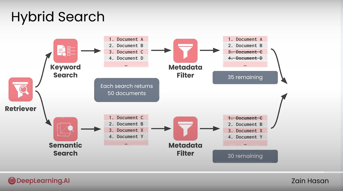 Overfetch + filter diagram — ANN search returning a large candidate pool (ef x filter_overfetch), then a metadata filter keeping only the qualifying subset, with arrows showing how the surviving results are re-sorted and truncated to k
Step 2: Score exactly. For every candidate ID the index returns, I fetch the full float32 vector and compute an exact similarity score using the configured metric. No approximation at this stage, even if the retrieval was approximate. The ANN index finds the right neighbourhood cheaply; the exact scoring happens on the small result set.
Step 3: Filter and truncate. If a metadata filter is present, it runs here against the scored hits. The filter is a chain of conditions with AND semantics:
Filter::new()
    .eq("language", "en")
    .gte("year", 2020)
    .is_in("category", vec!["science", "tech"])
Range, equality, not-equal, and set membership are all supported. This all happens in-process against the metadata stored in memory — no secondary I/O. After filtering, sort by score, truncate to , done.
SearchConfig: the recall/latency dial
Three named presets control how thoroughly the index is explored per query:
| Preset | ef (HNSW) | nprobe (IVF) | Use case |
|---|---|---|---|
fast | 50 | 1 | Batch pipelines, latency over recall |
balanced | default | default | General interactive RAG |
high | 400 | 20 | Compliance retrieval, precision-critical |
ef is the most important knob for HNSW. It sets the beam width for the layer-0 search: larger means the algorithm explores more of the graph before committing to a result set, which finds better neighbours but costs more CPU. A useful rule of thumb: at (for , : ) you typically see Recall@10 above 95%. Pushing to usually hits 99%+. Cost scales roughly linearly with .
| ef | Recall@10 (approx) | latency multiplier |
|---|---|---|
| 10 | ~85% | 1× |
| 50 | ~93% | 1.8× |
| 100 | ~96% | 2.5× |
| 200 | ~98% | 4× |
| 400 | ~99.5% | 7× |
You can override SearchConfig per request without touching the collection's default:
# collection config default
index:
  type: Hnsw
  ef_search: 200

# per-request override in SearchParams
search_config_override:
  ef: 400
That one query runs at ef=400 while everything else keeps running at the default. Useful when 99% of traffic is interactive RAG at balanced and an occasional compliance query needs high.
ef and overfetch interact. If you have a filter with
expansion = 5and request atef = 50, the engine runs HNSW with beam widthmax(ef=50, expansion*k=50) = 50and hands 50 candidates to the filter. Raising toef = 400gives the filter 50 candidates drawn from a much larger portion of the graph — better coverage of the eligible set for selective filters.
Filtered search and the selectivity problem
The hardest practical case in vector search is combining ANN with a highly selective metadata filter. I use in-traversal filtering for HNSW: filtered-out nodes are still used as graph traversal stepping stones but excluded from the result heap. This is better than naive post-filter because traversal keeps going until ef qualifying candidates are found rather than stopping at ef total candidates.
But for very selective filters (say, 1–2% of the dataset qualifies), even a large ef budget can't surface enough eligible candidates in one pass. Every hop in the graph is likely to land on a non-qualifying node. The filter_overfetch parameter is the practical knob here: set it to something like 50 for a 2% selective filter and you'll usually get enough hits. For < 1% selectivity, the right architecture is a purpose-built filtered index with separate entry points per filter attribute — that's on the roadmap. Longer term, I want the system to pick the overfetch multiplier automatically based on observed filter selectivity. That kind of self-tuning behavior — the database learning its own workload patterns rather than requiring manual configuration — is what I mean by making Piramid "natively smart."
Batch search and parallelism
For multiple queries at once, I route them through search_batch_collection, which reuses the same vector and metadata maps across the whole batch. When parallel_search is enabled, queries run in parallel via Rayon — which is one of my favorite Rust crates just for how little code it takes to get real parallelism:
if storage.config().parallelism.parallel_search {
    queries
        .par_iter()
        .map(|query| search_collection_with_maps(...))
        .collect()
}
Each query is independent and reads only immutable references to the vector store, so there's no locking in the hot path.