Embeddings
In the previous section I established that a vector database doesn't search for exact matches; it searches for geometric proximity in embedding space. That raises the obvious follow-up question: where do those vectors come from, and what does it actually mean for two vectors to be "close"? That's what this section is about.
I first truly understood how embeddings work when I took DAT 494 (Advanced Deep Learning) at ASU, where we covered tokenization, embedding layers, pretraining, and post-training from the ground up. But what really made it click was building things from scratch — I implemented language models from fundamentals covering Llama, KiVi, PaLiGemma, DeepSeek, and Mixtral, and taught 4 workshops on language model and RLHF engineering to 600+ attendees at AIS. Resources like Umar Jamil, Sebastian Raschka, 3Blue1Brown, and AI Engineering by O'Reilly were huge for building my intuition. I've collected all my learning resources here for anyone interested. The pretraining stage — tokenization and the embedding layer specifically — is where the geometry of these spaces truly clicked for me.
 embeddings
From words to numbers: why representation matters
Before neural embeddings, the standard way to represent text for information retrieval was bag-of-words or TF-IDF — and it's worth understanding why that broke, because it makes the whole point of embeddings obvious. A document becomes a sparse vector of length (the vocabulary size, typically 50,000–200,000), where component is some weight for word .
TF-IDF weights are:
This is fast and interpretable. The problem is that it's purely lexical — it has no notion of meaning. The words "car" and "automobile" are orthogonal vectors even though they mean the same thing. "Not good" and "bad" are distant even though they express the same sentiment. Any query about "machine learning" misses documents about "deep learning" or "neural networks" unless those exact words appear. Synonymy, polysemy, compositionality — TF-IDF breaks on all of them.
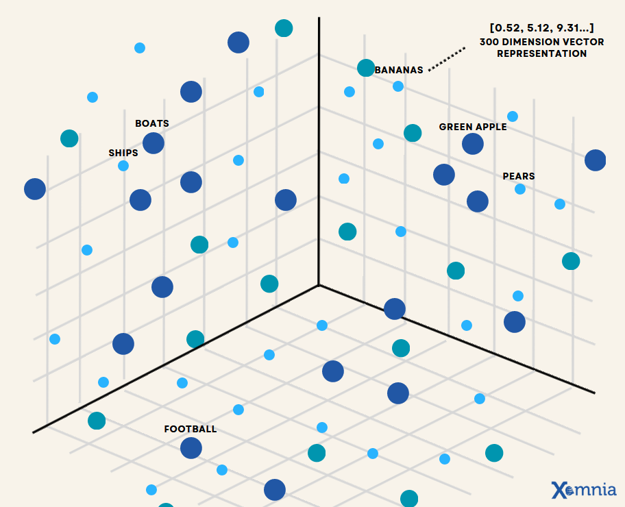
Distributed representations (embeddings) solve this by learning a dense -dimensional vector for each concept where the coordinates encode meaning, so similar meanings land near each other. The key insight is the distributional hypothesis: words that appear in similar contexts tend to have similar meanings. If you train a model to predict context from word (or word from context), the internal representations it must learn to do this successfully will encode semantic similarity as geometric proximity.
The manifold hypothesis: real-world data like text, images, and audio doesn't fill uniformly. It lies near a much lower-dimensional curved surface (a manifold) embedded in the high-dimensional space. A model that learns to embed sentences into is essentially learning a coordinate system on this manifold. Two sentences that are close on the manifold (semantically similar) map to nearby coordinates. This is why a vector can meaningfully represent the semantics of a sentence that might require thousands of words to fully describe: the manifold intrinsically has far fewer than 1536 degrees of freedom.
What an embedding actually is
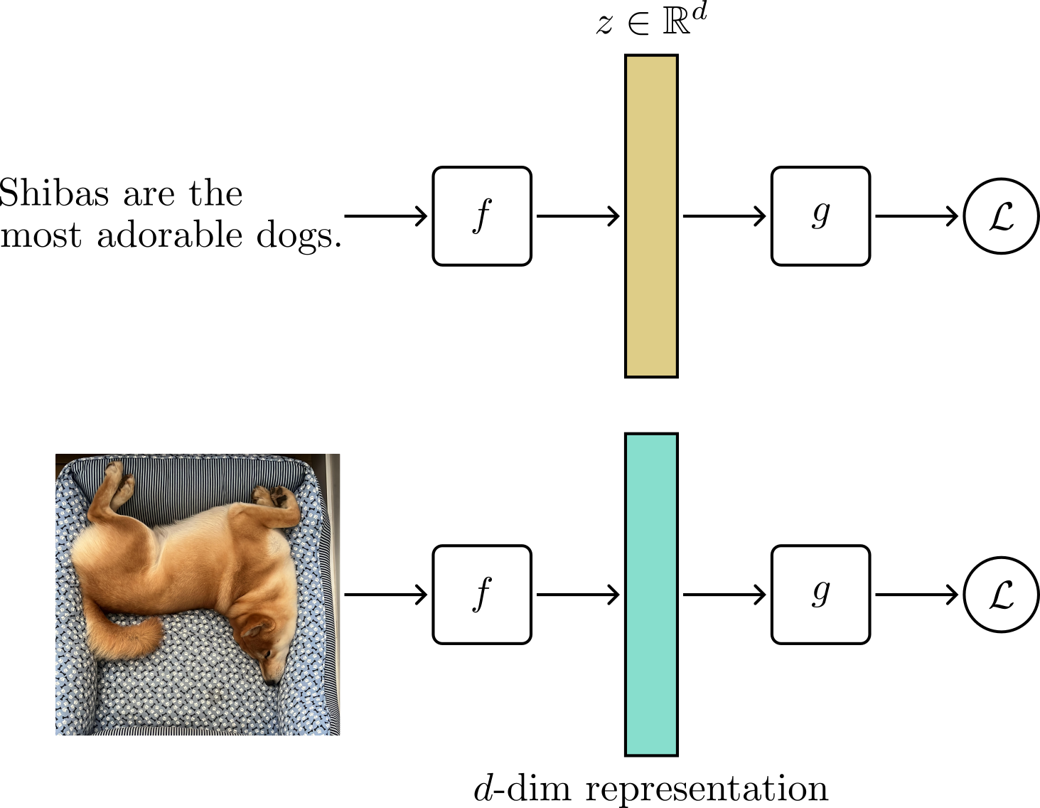
An embedding is a function that maps some input domain (text strings, images, audio clips) to a point in -dimensional real-valued space. The function is learned, not designed. A neural network is trained on large amounts of data with an objective that forces semantically related inputs to map to geometrically nearby points. Once trained, the network is frozen and its internal activations at some layer become the embedding vector.
Word2Vec and the skip-gram objective
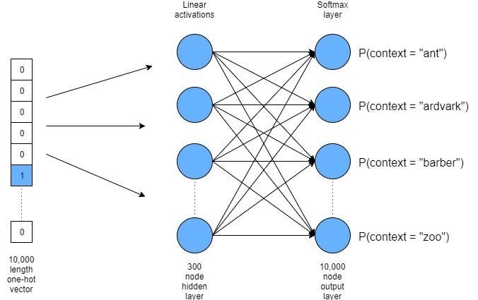
Word2Vec is the clearest example that makes this concrete — and it's worth working through even though modern models look nothing like it, because the intuition carries forward. The skip-gram variant trains a shallow neural network to predict context words from a center word within a window of size . The training objective maximises:
where is modelled via a softmax over all vocabulary words:
Here is the "input" embedding for word and is the "output" embedding for context word . The problem is that evaluating this softmax requires summing over all vocabulary members per training step, , which is prohibitively expensive at vocabulary sizes of 100K+.
The practical solution is negative sampling: instead of computing the full softmax, train a binary classifier that distinguishes the true context word from randomly sampled "noise" words. The objective becomes:
where is the sigmoid function and is a noise distribution (typically unigram frequency raised to the 3/4 power). This replaces with per update, with – in practice.
The gradients from this objective shape a 300-dimensional embedding space where words that appear in similar contexts end up near each other. The famous arithmetic — — falls out as an emergent property, not something explicitly built in. It reflects that the "royalty" direction and the "gender" direction are approximately linear in the learned space. That blew my mind when I first saw it.
 Word2Vec vector arithmetic — king − man + woman ≈ queen emerges naturally from training on context co-occurrence, not from any explicit encoding of gender or royalty
The word2vec arithmetic demo — royalty minus gender plus gender-swap lands near queen. It's a side effect of the geometry, not something that was explicitly designed in.
Word2Vec vector arithmetic — king − man + woman ≈ queen emerges naturally from training on context co-occurrence, not from any explicit encoding of gender or royalty
The word2vec arithmetic demo — royalty minus gender plus gender-swap lands near queen. It's a side effect of the geometry, not something that was explicitly designed in.
Word2Vec is a useful mental model but the limits become obvious fast. Each word gets exactly one vector regardless of context — so "bank" (financial) and "bank" (river) share the same point in space, which is obviously wrong. And it operates at the word level with no mechanism for whole sentences.
Transformers and contextual embeddings
Modern embedding models are transformer-based and address both limitations. If you've read the title "Attention is All You Need" (Vaswani et al. 2017) without really digging into it — this is the part that matters. The transformer's central mechanism is multi-head self-attention, which lets every token's representation be influenced by every other token in the sequence. So "bank" in "river bank" ends up near "water" rather than "finance", because the context shifts the representation.
For a single attention head with input matrix (where is sequence length), the computation is:
where , , are linear projections, and is the key dimension. The scaling factor prevents the dot products from growing large enough to push softmax into regions of vanishing gradient; without it, the softmax saturates and learning stalls.
Multi-head attention runs such operations in parallel with separate projections, then concatenates and projects the outputs:
With heads and (BERT-base), each head operates in dimensions. Different heads learn to attend to different types of relationships (syntax, coreference, semantic roles) simultaneously.
The result is that each token's output representation is a weighted mixture of all tokens' value vectors, with weights determined by how "relevant" each token is to the current one. This is the fundamental fix for Word2Vec's one-vector-per-word problem: the same token gets a different representation every time depending on what surrounds it.
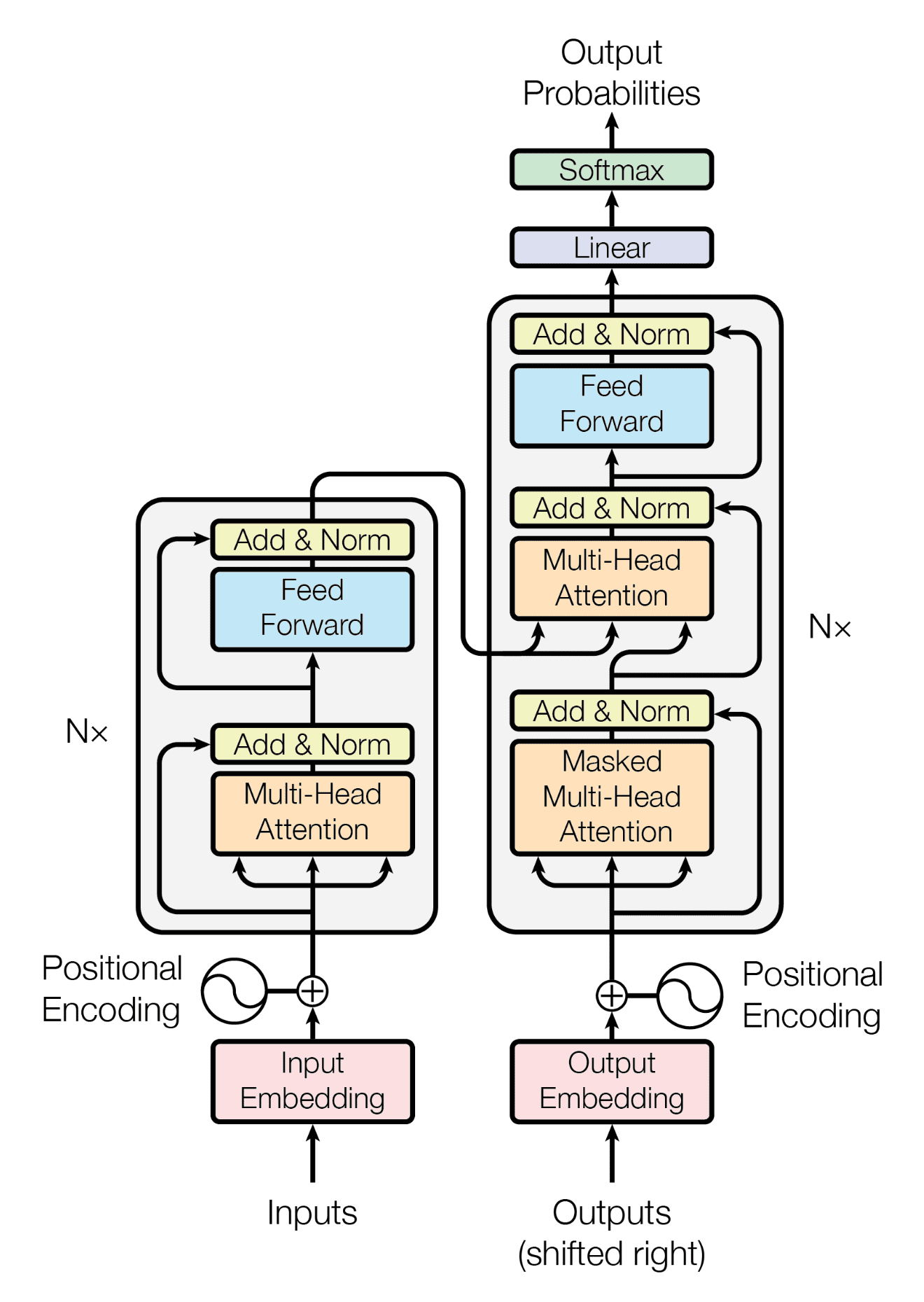 Transformer architecture — queries, keys and values flow through multi-head self-attention and feed-forward layers, with residual connections and layer norm at each step (Vaswani et al. 2017)
The original transformer from "Attention is All You Need" — queries, keys, and values run through multi-head attention and feed-forward layers with residual connections around each. The encoder half is what most embedding models use.
Transformer architecture — queries, keys and values flow through multi-head self-attention and feed-forward layers, with residual connections and layer norm at each step (Vaswani et al. 2017)
The original transformer from "Attention is All You Need" — queries, keys, and values run through multi-head attention and feed-forward layers with residual connections around each. The encoder half is what most embedding models use.
Positional encoding: transformers have no inherent notion of word order (unlike RNNs). Position is injected by adding a positional encoding to each token embedding before the first attention layer. The original formulation uses sinusoidal functions: , . Modern models use RoPE (Rotary Position Embedding) which encodes relative rather than absolute positions and generalises better to sequences longer than those seen during training.
To get a single embedding vector for an entire input text, most models either use the final-layer hidden state of a special [CLS] token inserted at the start of the sequence, or compute the mean pool of all token representations across the final layer:
Mean pooling treats all tokens equally; the CLS token approach trains the model to distil the full sequence meaning into that single position. Empirically, mean pooling tends to outperform CLS pooling on retrieval benchmarks when the model wasn't specifically trained with a CLS objective.
Contrastive learning: teaching similarity
Here's the part that isn't obvious at first: a pre-trained language model knows syntax and semantics, but that doesn't mean its internal similarity geometry lines up with what you want for retrieval. A GPT-style model trained on next-token prediction has representations useful for generation — not necessarily for finding similar documents. Contrastive fine-tuning is what reshapes that space specifically for similarity search, and it's why retrieval-specific models outperform general-purpose language models at this task.
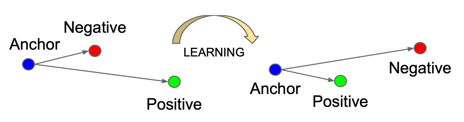
Contrastive training operates on pairs: a query and a positive (semantically related) and a set of negatives (unrelated). The standard loss is a variant of InfoNCE (Noise Contrastive Estimation):
where and are the normalized embeddings of a positive pair, and are all negatives in the batch. The temperature controls how sharply peaked the distribution is: small makes the model very sensitive to small distance differences (high contrast), while large allows more spread.
The denominator sums over all non-matching samples in the batch; this is in-batch negative sampling, and it's why larger training batch sizes produce better embedding models. With samples per batch, each training example is contrasted against 4095 negatives simultaneously. The signal from 4095 negatives is much richer than from a handful, forcing the model to learn a much stricter notion of "similar."
Hard negatives: the most effective training uses hard negatives, which are samples superficially similar to the query but subtly different (e.g., the same question paraphrased slightly, or a document from the same domain but a different topic). In-batch random negatives are mostly easy (a query about cooking vs a passage about finance is trivially distinguishable). Hard negatives force the model to develop fine-grained discriminative representations. Models like E5, GTE, and the OpenAI text-embedding-3 series are trained with hard negative mining pipelines; the measurable quality difference between them and earlier models is largely attributable to this.
Temperature calibration has a mathematically interesting role. The optimal isn't a fixed constant; it depends on the expected magnitude of similarity scores in your data. If your embeddings are -normalized (as is standard), cosine similarity ranges from -1 to 1. The InfoNCE loss with (a common value) turns this into an effective "temperature" for the distribution: values range from about -14 to +14, giving a reasonably peaked softmax. Too-small produces a distribution so sharp that small numerical errors dominate; too-large makes the loss insensitive to the exact relative ordering of candidates. OpenAI's models use a learned logit_scale parameter that plays the role of , optimising it jointly with the embedding weights during training.
 Contrastive training
The geometry of learned embedding space
A few geometric properties of embedding spaces are worth internalizing — they're what actually determines how you should configure distance metrics and quantisation, and I spent longer than I'd like to admit debugging recall issues before these clicked for me.
normalisation. Most production embedding models output -normalised vectors, each satisfying . On the unit hypersphere, cosine similarity and Euclidean distance are monotonically related:
So minimising L2 distance and maximising cosine similarity are equivalent for normalised vectors. The practical reason to normalise is that it makes similarity scores comparable across different inputs; unnormalised dot products are biased by vector magnitude, which correlates with input length and vocabulary frequency.
Anisotropy and dimensional collapse. Language models trained only with next-token prediction tend to produce anisotropic embedding spaces, where all vectors cluster in a narrow cone of the "occupied" subspace rather than spreading uniformly across . This was documented in the "BERT sentence embeddings" literature (Ethayarajh 2019, Li et al. 2020) and is measurable as a high average cosine similarity across random sentence pairs ( for vanilla BERT vs for a well-trained retrieval model). Contrastive fine-tuning pushes the embeddings toward isotropy, spreading them across the full surface of the unit sphere, which dramatically improves nearest-neighbour search quality.
Matryoshka Representation Learning (MRL). OpenAI's text-embedding-3 models use a training technique called MRL (Kusupati et al. 2022) that makes the embedding dimensions hierarchically meaningful. The full -dimensional vector is trained, but the loss is summed over a set of nested truncation sizes :
where is the first dimensions of the full embedding. This forces the model to pack the most discriminative information into the first few dimensions, with later dimensions adding progressively finer-grained signal. The practical benefit: you can truncate text-embedding-3-small's 1536-dimensional output to 512, 256, or even 64 dimensions and still get strong retrieval performance, with Recall@10 at 256 dimensions being only a few points below the full 1536d. This is a significant memory and compute saving when you control the tradeoff consciously.
Choosing dimensions with MRL: a useful heuristic for selecting the truncation size is to plot Recall@10 vs on a sample of your actual query/document pairs and find the elbow point. For most English text retrieval tasks, the elbow is around 256–512 dimensions. Going below 128 usually degrades recall noticeably, while going from 1024 to 1536 often gives less than 1 point of improvement. Only you can decide what tradeoff is right given your latency budget and recall requirements.
 Matryoshka Representation Learning — the first dimensions carry the most discriminative signal, so you can truncate the vector to any nested size and still get strong retrieval
MRL nests the learning objectives: each prefix of the vector is trained to work as a standalone embedding, so you can truncate at any supported size and still get competitive recall.
Matryoshka Representation Learning — the first dimensions carry the most discriminative signal, so you can truncate the vector to any nested size and still get strong retrieval
MRL nests the learning objectives: each prefix of the vector is trained to work as a standalone embedding, so you can truncate at any supported size and still get competitive recall.
Providers
Embedding generation is treated as a runtime concern: you configure a provider and model at startup, and Piramid handles the rest. I started with two provider types — OpenAI and local HTTP/TEI — because they're the most popular and the easiest to get running. I really want to add Cohere and Jina support too, but working alone on this entire project — code, SDKs, blogs, website — while juggling two research labs, a part-time job, two student orgs, and classes means I have to be ruthless about scope. More providers are coming. Both current providers implement the same Embedder trait:
#[async_trait]
pub trait Embedder: Send + Sync {
    async fn embed(&self, text: &str) -> EmbeddingResult<EmbeddingResponse>;
    fn provider_name(&self) -> &str;
    fn model_name(&self) -> &str;
    fn dimensions(&self) -> Option<usize>;
}
The dimensions() method lets downstream code validate that a stored collection's dimension matches the currently configured model before wasting compute on a mismatched embed+search cycle.
OpenAI
I support three models through the OpenAI provider:
| Model | Dimensions | Notes |
|---|---|---|
text-embedding-3-small | 1536 | MRL-trained; best cost/quality ratio |
text-embedding-3-large | 3072 | MRL-trained; 2× cost, ~5% better recall |
text-embedding-ada-002 | 1536 | Legacy; no MRL; kept for backward compat |
Requests hit https://api.openai.com/v1/embeddings with Authorization: Bearer {api_key} and encoding_format: "float" so you get raw float32 values directly. The API key is resolved from config.api_key first, then the OPENAI_API_KEY environment variable; the fallback to env var is intentional for containerised deployments where you don't want secrets in config files:
let api_key = config.api_key.clone()
    .or_else(|| std::env::var("OPENAI_API_KEY").ok())
    .ok_or_else(|| EmbeddingError::ConfigError("...".into()))?;
The base_url field can override DEFAULT_OPENAI_API_URL. This is primarily useful for pointing Piramid at an OpenAI-compatible proxy (Azure OpenAI, or other compatible proxies) without changing any other config.
One thing worth knowing about text-embedding-3-small vs text-embedding-3-large: the larger model produces higher-dimensional vectors with meaningfully better semantic resolution, but at 2× the API cost and 2× the in-memory storage per vector. For most RAG use cases I've seen, text-embedding-3-small at full 1536 dimensions or even at 512 (via MRL truncation) hits a good cost/quality balance. The legacy ada-002 exists for collections built before the v3 models.
Local HTTP and TEI
The local provider speaks to any OpenAI-compatible or TEI-style HTTP endpoint. TEI (Hugging Face text embeddings server) is Hugging Face's high-throughput embedding server; it exposes the same /embeddings JSON contract as the OpenAI API, making it a drop-in replacement. Ollama, TEI, and other locally-hosted embedding runtimes all work as long as they implement that protocol.
A typical local setup for TEI running a 768-dimensional model:
embeddings:
  provider: local
  model: BAAI/bge-base-en-v1.5
  base_url: http://localhost:8080/v1/embeddings
  timeout: 10
If you're already running a local model for generation, you almost certainly want embedding to be local too. Having both on the same machine eliminates the network round-trip and keeps your documents away from remote APIs entirely. A local TEI instance on a modern CPU can embed short texts in under 5ms, comparable to OpenAI API latency but without the variance of an external network call.
Model alignment: be careful about mixing embedding models across insert and search operations. If you insert documents with one model and then reconfigure the server to use a different model (different architecture, even same dimensionality), searches will produce nonsense results; the query embedding and the stored embeddings come from different spaces. There's no model-version locking per collection, so this is easy to do accidentally. Worth noting in production ops.
Configuration and resolution order
embeddings:
  provider: openai          # openai | local
  model: text-embedding-3-small
  base_url: ~               # required for local; overrides default for openai
  api_key: ~                # read from OPENAI_API_KEY env var if absent
  timeout: 30               # seconds; requests hang forever if absent
The resolution order for api_key is config file → OPENAI_API_KEY env var → error. Everything else comes only from the config file; there are no other environment variable overrides for model, base_url, or timeout. There's no per-request override for provider or model; the server uses whatever it was configured with at startup, and all collections on that server share the same embedding configuration.
The timeout field is important to set in production. If the embedding endpoint becomes unresponsive (OOM on the remote server, network partition, cold-start delay on a local model), Piramid's embed and search/text endpoints will block indefinitely without it. For OpenAI, 30 seconds is generous; normal latency is well under 500ms. For a local model running on CPU with a large context, you may need 60 seconds or more.
Request flow: /embed and /search/text
When you call POST /api/collections/{collection}/embed, Piramid takes your text, routes it through the configured embedder stack, and stores the resulting vector. POST /api/collections/{collection}/search/text does the same for the query text; it's embedded on the fly and then passed into the ANN search path.
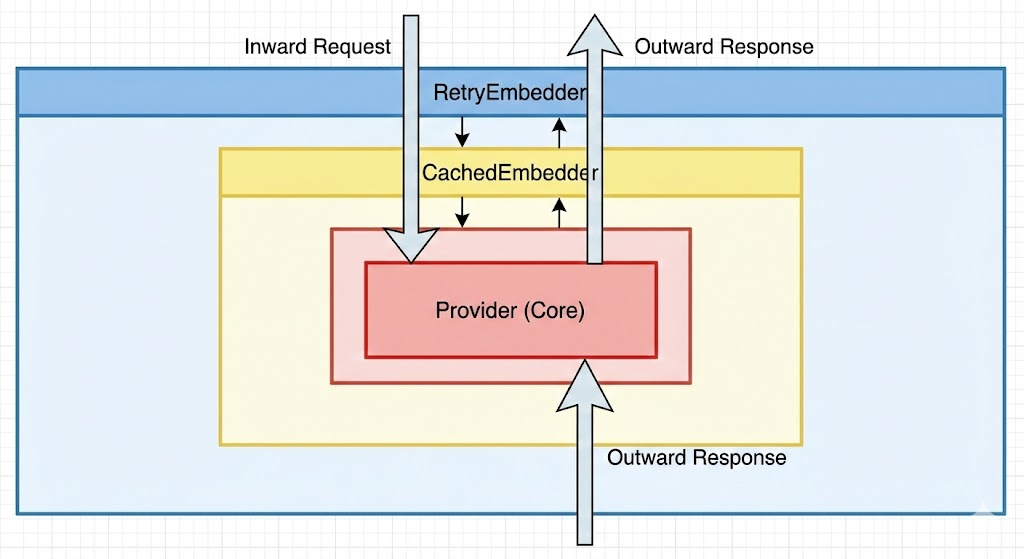
I structured the embedder stack as three layers:
Request
  └── RetryEmbedder          (exponential backoff on transient failures)
        └── CachedEmbedder   (LRU cache, default 10K entries)
              └── Provider   (OpenAIEmbedder or LocalEmbedder)
 Embedder Stack
This stack exists because things break in practice. I learned this the hard way — during a demo of SparkyAI in front of my professor, the embedding provider hit a cold start timeout and the whole system just froze. I had to fall back to a local model on the spot. After that I decided any embedding layer I build needs retry logic baked in, not bolted on.
Embedder Stack
This stack exists because things break in practice. I learned this the hard way — during a demo of SparkyAI in front of my professor, the embedding provider hit a cold start timeout and the whole system just froze. I had to fall back to a local model on the spot. After that I decided any embedding layer I build needs retry logic baked in, not bolted on.
The ordering is deliberate. I put the cache inside the retry wrapper: if the underlying provider fails on the first attempt, the retry wrapper fires, but a subsequent cache hit will short-circuit before hitting the provider again. A cache miss falls through to the provider, and the result gets stored in the LRU on the way back up. Every layer is transparent to the caller; all three implement the same Embedder trait.
I key the cache on the exact raw text string. Identical inputs across different collections on the same server share the same cache entry. This is intentional: if the same document appears in multiple collections, the embed call is only paid once per server lifetime (until eviction). The tradeoff is that the cache is semantically unaware: "computer science" and "CS" are different keys even though they'd produce nearby vectors. A semantic-deduplication cache would be more memory-efficient for collections with near-duplicate content, but adds significant complexity.
Retry and error classification
The RetryEmbedder uses exponential backoff with: initial_delay = 1000ms, doubling each attempt, capped at max_delay = 30,000ms, max_retries = 3.
Not all errors are retried. The is_retryable_error function classifies errors before deciding:
fn is_retryable_error(error: &EmbeddingError) -> bool {
    matches!(error,
        EmbeddingError::RateLimitExceeded | EmbeddingError::RequestFailed(_))
    // AuthenticationFailed is NOT retried — retrying with a bad key is pointless
}
A 401 authentication failure propagates immediately: no delay, no retry. A 429 rate limit or a connection error retries with backoff. After exhausting all retries, the last error propagates up as a 5xx from the Piramid API.
The embedding provider is also a health endpoint.
GET /api/health/embeddingschecks whether the configured provider is reachable and responding. A failing embedding provider will surface there before it causes query failures, worth monitoring in production alongside standard CPU/memory metrics.
The caching tradeoff
The LRU cache holds up to 10,000 embeddings by default. Each text-embedding-3-small vector is bytes. A full 10K-entry cache occupies roughly 60MB, a manageable overhead relative to the collection's vector storage.
Cache effectiveness is entirely workload-dependent:
High hit rate: a RAG system where a fixed corpus is loaded at startup and then queried repeatedly. After the first pass over the corpus, every document re-embed on restart hits the cache, eliminating API calls entirely during warm-up. Effective cache size is .
Near-zero hit rate: a system where every input is a unique real-time user query. Each query is distinct, the cache never hits, and the overhead is a lock acquisition per request (the CachedEmbedder wraps access in a Mutex<LruCache>). That's a few hundred nanoseconds per call, not worth worrying about.
The eviction boundary matters: if your hot corpus has 12,000 documents and the cache holds 10,000, the oldest 2,000 entries get continuously evicted and re-fetched. This is a surprising cliff effect; the 10K default works well for corpora that fit, and degrades suddenly for slightly larger ones. If you have a fixed corpus, set the cache size to corpus_size + 20% to avoid thrashing.
One thing the cache doesn't do is persist across restarts. It is in-memory only. A server restart means re-embedding your entire corpus on the first pass. For large corpora on paid embedding APIs, this can be a non-trivial cost. A persistent embedding store (write the vectors to a separate key-value store keyed by content hash) is a common production pattern to address this.
Dimensions, memory, and the cost of scale
A collection with vectors of dimension stored as float32 requires exactly bytes.
For , (OpenAI text-embedding-3-small):
For text-embedding-3-large at the raw storage doubles to 12.3 GB. These numbers don't include the index structure; HNSW adds roughly another 550 MB of edge storage for vectors at (see the indexing section for the derivation). Total working memory is:
| Model | Vectors | Raw storage | + HNSW index | Total | |
|---|---|---|---|---|---|
| small | 1536 | 1M | 6.1 GB | 0.55 GB | ~6.7 GB |
| large | 3072 | 1M | 12.3 GB | 0.55 GB | ~12.8 GB |
| small | 1536 | 10M | 61 GB | 5.5 GB | ~67 GB |
These are the numbers that motivate quantisation and dimensionality reduction.
int8 scalar quantisation
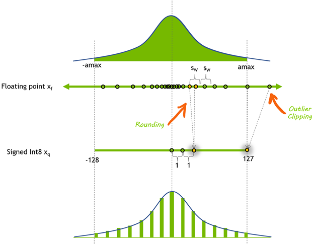 int8 quantisation diagram — a float32 range mapped linearly to 256 integer buckets, with the uniform step size ε_q shown as the gap between original float value and its nearest quantised level
Piramid supports int8 scalar quantisation, which compresses each float32 component to a signed int8 by linearly mapping the observed range:
Storage drops from to bytes per vector, a 4× reduction. Quantisation error introduces a small amount of distance measurement error. The distance error for a quantised component is bounded by the quantisation step size:
For -normalised embeddings, each component has range roughly (most of the variance is absorbed by the length-1 constraint spreading across 1536 dimensions), so . The total L2 distance error accumulated over components is approximately , small relative to typical inter-cluster distances.
When to use quantisation: int8 is appropriate when recall degradation is acceptable (< 1–2 pp Recall@10 drop for most datasets) and memory is the binding constraint. It is not appropriate when precision is critical: compliance retrieval, exact deduplication, or narrow similarity thresholding. For those workloads, keep full float32.
I started with int8 rather than fp16 or bfloat16 because it was the simplest to implement and gives the most dramatic compression ratio for an MVP. The goal isn't to lock users into one quantization format — I want this to be fully configurable, with fp16 and bfloat16 as future options. But for getting something working that I could demo and benchmark, int8 with a 4× reduction was the obvious first step. I've focused on writing modular code so adding more quantization variants is a matter of implementing additional formats, not restructuring the whole storage layer.
MRL truncation: a cleaner memory/quality tradeoff
For text-embedding-3 models, MRL truncation is often a better choice than quantisation for reducing memory. Truncating from 1536 to 512 dimensions is a 3× reduction with typically less recall degradation than int8 quantisation, because you're discarding the least-informative dimensions rather than uniformly degrading all of them.
The approximate recall retention curve for text-embedding-3-small:
| Dimensions | MTEB Recall@10 (approx) | Memory vs full |
|---|---|---|
| 1536 | 100% (baseline) | 1× |
| 512 | ~97% | 3× savings |
| 256 | ~94% | 6× savings |
| 64 | ~85% | 24× savings |
Combining MRL truncation (e.g. to 512) with int8 quantisation gives a 12× memory reduction with recall typically staying above 95%, a practical configuration for memory-constrained deployments.
I apply quantisation at the storage layer rather than at embedding time. The full float32 vector is returned by the provider and stored, and quantisation is applied when writing to disk. This means the HNSW index always operates on full-precision vectors in memory while only the persistent storage benefits from compression. Full PQ integration (operating the ANN search on compressed codes) is on the roadmap and would reduce in-memory vector storage by 32× on top of the index savings; see the indexing section for the full memory math.