Indexing
A vector database without a good index is just a very sophisticated for loop. The core problem is this: given a query vector and a collection of stored vectors, find the closest by some distance metric. The naïve approach scans every vector and computes the distance, per query. At with (OpenAI's text-embedding-3-large), that is 1.5 billion multiply-accumulate operations per query. Even with SIMD, you're looking at tens of milliseconds. That is fine for batch analysis; it is not fine for a latency-sensitive RAG pipeline that needs sub-millisecond retrieval.
I built three index types — Flat, IVF, and HNSW — with an Auto mode that picks the right one based on collection size. Each represents a different point on the exact recall / query latency tradeoff curve.
Measuring quality: Recall@k
Before talking about how indexes work, it helps to be precise about what "good" means. The standard metric is Recall@k: the fraction of the true nearest neighbours that your ANN index actually returns.
A Recall@10 of 0.95 means 9.5 out of 10 returned results are genuinely in the top-10 by exact distance, meaning you missed half a result on average. For RAG, a downstream model consuming the top-5 retrieved chunks rarely produces a noticeably worse answer if one chunk is an 11th-nearest rather than a 9th-nearest neighbour. The semantic delta is tiny. This is why targeting Recall@10 ≥ 0.95 is reasonable for production and you should not sacrifice 2–3× query latency chasing 0.99.
The recall-latency frontier: every ANN algorithm traces a curve when you sweep its quality parameters. More recall always costs more latency. The goal of index design is to push that frontier as far to the upper-left (high recall, low latency) as possible. HNSW currently has the best-known frontier for general dense vectors at high dimensions.
Why high-dimensional spaces break classical indexes
The reason I didn't use a B-tree or even a kd-tree in Piramid isn't laziness — it's that those structures provably collapse at high dimensionality. Understanding why is important context before looking at HNSW and IVF, because otherwise "graph-based index" sounds like an arbitrary choice.
The kd-tree and why it fails
A kd-tree partitions by recursively splitting on alternating axes. At or it's an elegant exact nearest-neighbour structure with average query time. At — the space I'm actually working in — it's slightly worse than a random scan. The geometry breaks in a very specific way.
The key quantity is the volume ratio of a hypersphere to its enclosing hypercube. In dimensions, the volume of a unit ball is:
This goes to zero as . Practically, almost all the volume of a high-dimensional hypercube concentrates in its thin outer shell rather than its interior. An ANN query at radius around a point picks up essentially no volume, which means the kd-tree's bounding boxes contain almost no useful structure. The algorithm has to back up and explore essentially every branch, making the expected query complexity in the worst case, which at is worse than brute force.
Intuition for the shell concentration: In dimensions, the fraction of a unit ball's volume that lies within distance of the surface is . At and , this is , essentially all of the ball is shell.
Ball trees, cover trees, and R-trees all hit the same underlying problem. Any space-partitioning structure that works by dividing into regions will find that a query hypersphere at high intersects almost every region, destroying the logarithmic speedup.
Locality Sensitive Hashing
LSH takes a different approach: rather than partitioning space, it probabilistically maps similar vectors to the same hash bucket, then only computes exact distances within a bucket. It was the dominant ANN approach circa 2010–2014 before HNSW came along, and the core idea is still elegant. For a good hash family, the collision probability is a decreasing function of distance:
For random hyperplane LSH (the standard choice for cosine similarity), the collision probability between two unit vectors is:
To achieve recall with independent hash tables and bits per table, you need:
where is the collision probability at your target distance. This is workable but requires many hash tables (memory multiplier), and the constant factors are large. LSH dominated ANN benchmarks circa 2010–2014 but was comprehensively beaten in recall/latency/memory by HNSW once that paper appeared in 2016. The gap isn't close.
The curse of dimensionality, formally
The core issue underlying both failures has a formal name: the concentration of measure. For vectors drawn uniformly from the unit hypercube in , the ratio of the maximum to minimum distance from a query point converges to 1:
When all distances are nearly equal, there's no local structure for a spatial index to exploit — every point is equidistant from every other. In practice at real embeddings are far from uniformly distributed (they cluster by topic and semantics, because that's what the model was trained to do), which is why ANN indexes still work. But the observation explains why cosine similarity outperforms raw Euclidean distance for text: normalising away magnitude removes one whole axis of spurious distance variation.
What actually works at high dimensions: graph-based indexes (HNSW) exploit the empirical cluster structure of the data directly rather than trying to partition abstract coordinates. Quantisation-based indexes (IVF + PQ) exploit the fact that even high-dimensional vectors often lie near a much lower-dimensional manifold. Neither tries to fight the geometry of directly.
 Curse of dimensionality — as dimensions grow, all pairwise distances concentrate around the same value and spatial indexes lose their ability to prune the search space
As grows, all points collapse to roughly the same distance from any query — which breaks every partitioning assumption that spatial indexes rely on.
Curse of dimensionality — as dimensions grow, all pairwise distances concentrate around the same value and spatial indexes lose their ability to prune the search space
As grows, all points collapse to roughly the same distance from any query — which breaks every partitioning assumption that spatial indexes rely on.
Why approximate is good enough
This is a question I thought about a lot when building Piramid. Intuitively, "97% recall" sounds like a compromise. But when you look at what you're actually doing with the results, the math changes.
For RAG pipelines it almost never does. A retrieval consumer typically uses 5–20 retrieved chunks. If one of them is a 12th-nearest-neighbour rather than the 10th, the generated answer is unchanged with very high probability — the semantic gap between the 10th and 12th most similar vectors is essentially imperceptible. The accuracy loss from a well-configured HNSW index is typically 1–5%, and the query latency improvement over exact search is 10–100×.
Where recall does matter: deduplication (you need exact matches, not approximate ones), compliance retrieval (must surface every relevant document), and similarity thresholding (returning "no match" for queries below a distance cutoff requires precise distances). For those workloads, Flat or a post-search exact reranker is appropriate.
Flat: the honest baseline
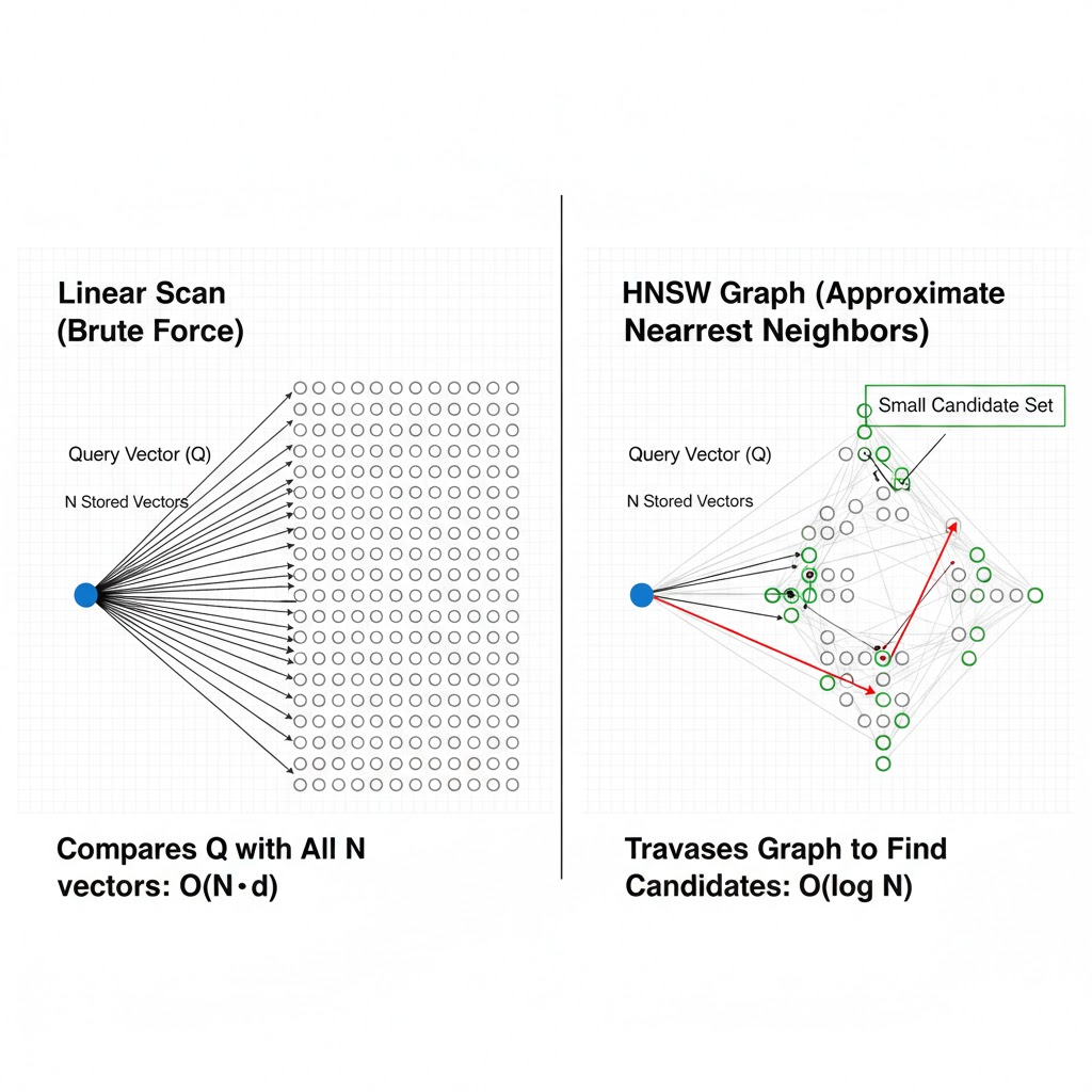 Linear scan illustration — a query point on the left, arrows fanning out to all N stored vectors, labeled O(N·d); contrasted with the HNSW graph on the right showing only the small candidate set explored during traversal
The Flat index does not pretend to be smart. For every query it iterates over every known vector ID, computes the configured similarity score, then returns the top in time. There is no build phase, no build memory overhead, and recall is exactly 1.0 by definition.
pub struct FlatIndex {
    config: FlatConfig,
    vector_ids: Vec<Uuid>,
}
That's the entire structure. The actual vectors live in the storage layer's HashMap; the flat index only holds the ordered list of IDs it has seen. The insert path is amortised (vector append), the remove path is (linear retain), and search is .
Why flat is fast at small N
Modern CPUs can execute SIMD dot products over f32 arrays at roughly 16 multiply-accumulates per clock cycle on AVX2 (8 f32 lanes × 2 fused multiply-add ports). At and 3.5 GHz, a single dot product takes on the order of:
Ten thousand such products take about 270 µs, squarely in the budget for a 1 ms response time. The entire dataset at and occupies , which fits comfortably in L3 cache on modern server CPUs (typically 32–96 MB). Once the working set is cache-warm, the scan is purely compute-bound rather than memory-bound, and the theoretical throughput is close to SIMD-peak.
SIMD warm cache vs cold: the first scan after startup is memory-bound, reading 61 MB from RAM (~40 GB/s) in roughly 1.5 ms. Subsequent scans of the same warmed cache hit at L3 bandwidth (~300 GB/s) and finish in ~200 µs. Piramid's warming phase at startup (described in the storage post) is partly motivated by this: you want the first real user query to hit warm memory, not cold RAM.
The crossover point where flat becomes clearly slower than an ANN index depends on both and . At , the flat scan stays competitive up to ~100K vectors because the vectors are smaller, the cache fits more of them, and the dot products are cheaper. At (some multimodal embeddings), the crossover arrives earlier since the 4× larger vectors mean 4× less fit in cache and 4× more compute per scan.
Piramid's auto-selector threshold of 10,000 is deliberately conservative: it leaves headroom for the case where the server's L3 is shared with other workloads.
HNSW: navigating a small world
HNSW (Hierarchical Navigable Small World, Malkov and Yashunin 2018) is the algorithm at the core of most high-performance vector databases — Pinecone, Weaviate, Milvus, and the Qdrant I used for years before building this. The intuition comes from graph theory's small-world phenomenon: in certain natural and engineered networks, the average shortest path between any two nodes grows only as even as becomes very large. HNSW constructs exactly this kind of network over your vectors and traverses it greedily during search.
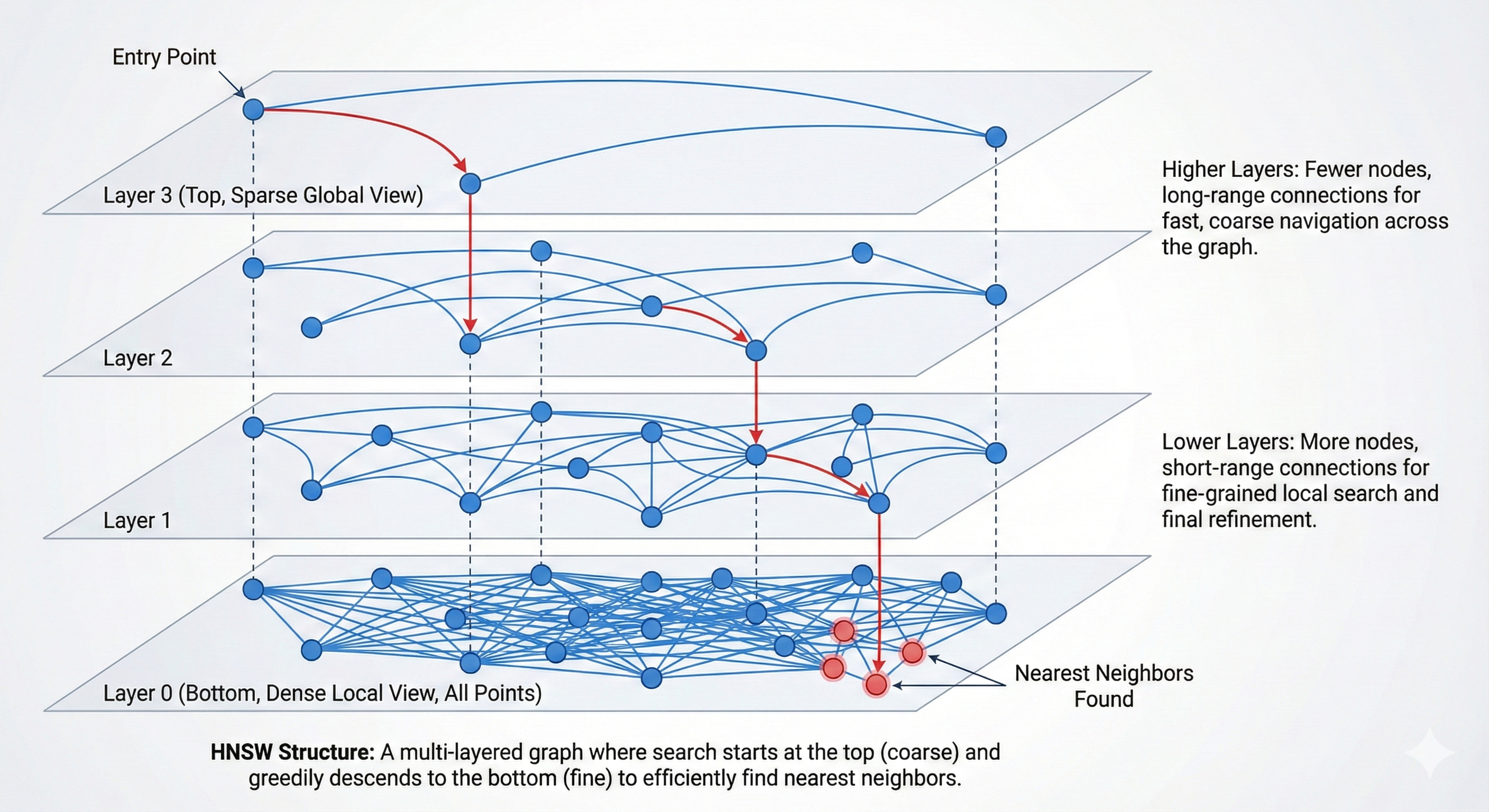 HNSW layered graph — layer 2 is sparse for long-range navigation, layer 1 is denser, layer 0 holds all nodes with the full connection density; search descends from top to bottom
HNSW layers: the top is a sparse express lane for long-range jumps, and each lower layer adds more nodes and edges until layer 0, which has everything. Search descends from top to bottom.
HNSW layered graph — layer 2 is sparse for long-range navigation, layer 1 is denser, layer 0 holds all nodes with the full connection density; search descends from top to bottom
HNSW layers: the top is a sparse express lane for long-range jumps, and each lower layer adds more nodes and edges until layer 0, which has everything. Search descends from top to bottom.
The small-world graph idea
The NSW (non-hierarchical) paper by Malkov et al. (2014) showed something counterintuitive: if you build a graph where each vector-node is connected to its approximate nearest neighbours plus a few "long-range" links to far-away nodes acting as shortcuts, greedy search on that graph finds nearest neighbours in hops with good probability.
Each node starts with short-range connections to similar vectors, forming local clusters. The long-range edges emerge naturally from the construction order: vectors inserted early (when the graph was sparse) connect to whatever was available at the time, spanning large distances. Late insertions find dense local neighbourhoods. The combination produces the small-world property — and it falls out from the construction process rather than being explicitly engineered in.
Greedy search simply starts from an arbitrary entry node and repeatedly moves to whichever of the current node's neighbours is closest to the query. It terminates when no neighbour is closer than the current node — a local minimum that empirically is almost always the global minimum for typical embedding distributions.
The raw NSW problem is that the entry point matters a lot. Starting in the wrong region wastes many hops just navigating to the relevant part of the space. HNSW solves this with a hierarchy of layers: layer 0 is the dense local graph, and each higher layer is a progressively sparser navigation structure that lets you coarsely zoom to the right region before descending into the dense layer.
Layer probability and occupancy
Every newly inserted vector is assigned a maximum layer drawn from a geometric distribution:
This gives . In other words, about of all vectors reach layer 1, reach layer 2, and so forth. The expected number of nodes at layer or above is:
With and : layer 0 has all 1M nodes, layer 1 has ~62,500, layer 2 has ~3,906, layer 3 has ~244. The total across all layers is:
So the multi-layer structure adds only about 6.7% overhead over storing the base layer alone. The hierarchy is nearly free in terms of node count.
fn random_layer(&self) -> usize {
    let r: f32 = rand::random();
    (-r.ln() * self.config.ml).floor() as usize
}
The default Piramid config is m = 16, m_max = 32 (layer 0 gets connections because it needs to be denser to handle the full nodes), ef_construction = 200.
Inserting a vector: the two-phase algorithm
Insert is a top-down descent followed by a bottom-up connection phase.
Phase 1: find the entry region. Starting from the global entry point (the node with the highest , which governs the top layer), the algorithm greedily descends from the top layer to . At each layer in this descent, it performs a greedy 1-nearest-neighbour search, just to find which part of the space to descend into. At the end of phase 1 you have a candidate entry point at the new node's target layer that is already in the right neighbourhood.
Phase 2: connect at each layer. From layer down to layer 0, the algorithm runs a richer ef_construction-nearest-neighbour search, maintaining a candidate priority queue of the best ef_construction results seen so far. From those candidates it selects the best (or at layer 0) and adds bidirectional edges:
for lc in (0..=layer).rev() {
current_entry = self.search_layer(vector, ¤t_entry,
self.config.ef_construction, lc, ...);
let m = if lc == 0 { self.config.m_max } else { self.config.m };
let neighbors = self.select_neighbors(¤t_entry, m, vectors, vector);
for &neighbor_id in &neighbors {
// add new_node → neighbor edge
pending_connections[lc].push(neighbor_id);
// add neighbor → new_node edge (bidirectional)
neighbor.connections[lc].push(id);
// prune neighbor's list back to m if it exceeded
if neighbor.connections[lc].len() > m {
neighbor.connections[lc] = self.select_neighbors(..., m, ...);
}
}
}
The bidirectionality is critical. A unidirectional graph would have large "dead end" regions, where nodes that many others point to have no useful outgoing edges. Bidirectional edges guarantee that traversal can always go in both directions, which is what makes the small-world property hold under greedy descent.
After adding the back-edge, if the neighbour's connection list exceeds , it gets pruned back. I went with simple distance-based selection: keep the closest. The original HNSW paper proposes a diversity-aware heuristic that prefers candidates spread across different directions, which improves recall slightly but adds implementation complexity. Piramid's simple greedy selection works well in practice.
Time complexity per insert is , where the comes from the number of layers, from the connections per layer, and from the width of each layer's search.
The beam search: formal invariant
The core of both insert and query is search_layer, which runs on a single layer. Understanding it precisely is important because ef is the main tuning knob exposed to users.
The algorithm maintains two data structures simultaneously:
- A candidates max-heap ordered by negative distance (so the top element is the closest candidate yet explored)
- A nearest max-heap ordered by distance (so the top element is the furthest among the current best results)
The invariant at each step: nearest holds the ef best nodes seen so far; candidates holds nodes whose neighbours haven't been explored yet that might still improve the result. The loop runs while there exist unexplored candidates closer to the query than the current furthest result:
while let Some(candidate) = candidates.pop() {
    if candidate.distance > furthest_distance { break; }
    for &neighbor_id in &node.connections[level] {
        if visited.insert(neighbor_id) {
            let dist = self.distance(query, neighbor_vector);
            if dist < furthest_distance || nearest.len() < num_closest {
                candidates.push(neighbor);
                nearest.push(neighbor);
                if nearest.len() > num_closest { nearest.pop(); }
                furthest_distance = nearest.peek().map(|c| c.distance)...;
            }
        }
    }
}
The termination condition candidate.distance > furthest_distance is key: once the closest unexplored candidate is already farther than our worst current result, expanding it can only add worse results, so we stop. This makes the algorithm output-sensitive: dense clusters terminate quickly (they fill nearest fast and tighten furthest_distance fast), while sparse regions iterate longer.
ef_construction vs ef_search
These two parameters are often confused because they both show up as ef internally, but they do completely different things.
ef_construction controls graph quality at build time. It is the beam width used during search_layer while inserting; higher values mean each new node finds better neighbours, resulting in a denser and more accurate graph. The cost is per layer per insert. Setting ef_construction = 200 means each insertion explores up to 200 candidates to find the best neighbours to connect to.
ef_search controls query recall at query time. It is the beam width for the final layer-0 search. It does not affect the graph structure at all, only how thoroughly the already-built graph is explored during a query. You can set ef_search = 50 at query time on a graph built with ef_construction = 400 without any degradation to the graph itself.
The practical implication: build with high
ef_construction(200–400) and tuneef_searchper use case. A graph built withef_construction = 64and queried withef_search = 400will never match the recall of a graph built withef_construction = 400and queried withef_search = 200— because the underlying graph just doesn't have the connections needed. Build quality is permanent. Search quality is adjustable.
Both default to 200. Override ef_search per query via SearchConfig:
collection:
  index:
    type: Hnsw
    m: 16
    ef_construction: 200
    ef_search: 200  # tune this at query time
At these settings, empirical Recall@10 on typical text embedding distributions is 97–99%.
Memory footprint of the graph
Each node in the HNSW graph stores:
- One
Vec<Vec<Uuid>>of connections across all its layers. A node at layer 0 only has connections; a node at layer 1 has more; and so on. - A
tombstone: boolflag (1 byte).
The expected total storage for connections is:
With , , : roughly . That is on top of the raw vector storage (). The graph overhead is about 9% of vector memory, a modest tax for the search speedup.
Tombstoning and graph connectivity
Deletion in graph-based indexes is notoriously awkward. Physically removing a node and its edges can disconnect parts of the graph; future traversals may fail to reach regions that were only accessible through the removed node. This is not a theoretical concern: if a hub node (one that happens to be the entry path to an entire cluster) is deleted and its edges removed, searches into that cluster will silently produce incorrect results.
I went with tombstoning after seeing the alternative up close. I met a member of the SuperMemory team once who showed me their agentic knowledge graphs — they were doing full node deletion with LRU eviction, rebuilding the entire graph structure every time nodes were removed. The overhead was enormous. Rebuilding an entire index on the spot just because of one deletion is insanity. The analogy I keep coming back to is how Instagram handled the likes feature — they optimized the UX and accepted some technical sacrifice behind the scenes, and the result was great. People are the actual product. So a deleted node has its tombstone flag set to true but its edges are kept intact in memory.
fn mark_tombstone(&mut self, id: &Uuid) {
    if let Some(node) = self.nodes.get_mut(id) {
        node.tombstone = true;
    }
}
During search, tombstoned nodes are used as traversal intermediaries; their edges are still followed when exploring the graph, but they are filtered out before the result set is returned. This guarantees graph connectivity at the cost of retaining dead nodes in memory.
Tombstone accumulation risk: if a workload has high delete rates, tombstones pile up. The graph's "live density" (the number of non-tombstoned nodes per layer) gradually decreases, and eventually traversal is slow because a large fraction of the explored nodes are dead weight. The fix is a full index rebuild from the live vectors, which Piramid triggers through its compaction mechanism. After compaction, the loaded index is a clean graph with no tombstones.
IVF: Voronoi cells and k-means
IVF partitioned vector space
IVF partitions the vector space into Voronoi cells via k-means. At query time only the closest
nprobe cells are scanned, limiting the search to a small fraction of the dataset.
IVF (Inverted File Index) takes a completely different approach to the ANN problem. Rather than building a navigable graph, it partitions the vector space into clusters using k-means, and for each cluster maintains an inverted list (the IDs of vectors assigned to that cluster). At query time it only scans the nprobe closest clusters rather than everything.
The geometric picture is a Voronoi diagram. Each centroid defines a cell:
A query vector falls into the cell whose centroid is nearest. Probing nprobe clusters means searching the query's own Voronoi cell plus the adjacent cells, the ones whose centroids are next-closest to . Any true nearest neighbour that lies near a cell boundary may exist in an adjacent cell, which is the fundamental recall limitation of IVF with small nprobe.
Building the clusters: Lloyd's algorithm
Centroid computation uses Lloyd's k-means algorithm:
- Initialise: pick vectors at random as initial centroids .
- Assign: for each vector , find its nearest centroid: .
- Update: recompute each centroid as the mean of its assigned vectors: .
- Repeat steps 2–3 until convergence or
max_iterations.
I run 10 iterations by default. Lloyd's algorithm minimises the within-cluster sum of squared distances (inertia):
Each iteration monotonically decreases , so convergence is guaranteed. In practice the large gains come in the first 3–5 iterations; later iterations move centroids by tiny amounts. Ten iterations is a reasonable engineering tradeoff between cluster quality and startup cost.
k-means++ vs random initialisation: Piramid uses random initialisation (just takes the first vectors). k-means++ initialises centroids by sampling proportionally to , which produces better initial spread and usually converges in fewer iterations. It's a potential improvement to the build phase for distributions where random initialisation produces early clustering near dense regions.
Why K ≈ √N is optimal
The total cost of an IVF query is:
where is the cost per centroid distance computation and is the cost per vector distance computation inside the inverted list. To minimise over (treating nprobe as fixed at 1), take the derivative and set to zero:
Since (both are dot products of similar-dimensional vectors with the same SIMD path), we get . That's where my auto-config for IVF comes from:
pub fn auto(num_vectors: usize) -> Self {
    let num_clusters = (num_vectors as f32).sqrt().max(10.0) as usize;
    let num_probes = (num_clusters as f32 * 0.1).max(1.0).min(10.0) as usize;
    ...
}
At : , num_probes = 10. Average cluster size is vectors. A query scans vectors, a 32× reduction over the full scan, with recall typically around 95%.
At this optimal , the total query cost is (verify: ). Compare to flat scan at : IVF is times the flat cost, so the speedup factor scales as . At , that's a theoretical 500× speedup over flat; in practice you get 50–100× because of cache effects and overhead.
The cluster boundary problem
The recall degradation with small nprobe comes from vectors that land near cell boundaries. If your nearest neighbour and your query are separated by a Voronoi boundary, the true nearest neighbour is in a different cluster than the one containing the query. With nprobe = 1, it is missed.
How common is this? For uniformly distributed points, the expected fraction of a dataset that lies near any boundary scales roughly as , essentially 100% at high dimensions, because every vector is near some boundary (again, concentration of measure). For real embedding distributions which are manifold-like rather than uniform, the fraction is much smaller because the data has strong cluster structure.
This is why IVF works poorly for synthetic uniform distributions in benchmarks but works well on real embedding datasets: semantic structure means vectors genuinely separate into clusters, and boundaries are relatively sparse in the data-dense regions.
Online insertion and cluster drift
After the clusters are built, new vectors are assigned to the nearest existing centroid and appended to that inverted list. No re-clustering happens. This is correct for stationary data distributions, but if the distribution shifts over time (new document topics, new languages, a different embedding model) some clusters become overloaded (recall degrades because the list is too long) and others become nearly empty (throughput degrades because you're scanning small irrelevant lists). The nprobe budget buys you decreasing recall per probe when clusters are imbalanced.
The fix is a periodic rebuild: re-run k-means on the current live vector set, reassign all vectors to new centroids, and reconstruct the inverted lists. I trigger this through the compaction mechanism, exactly as with HNSW graph rebuilds.
Where this is headed: I haven't run formal benchmarks between HNSW and IVF yet — I've been focused on building features and keeping the codebase clean. I expect HNSW to dominate on 100K+ vector datasets in latency, but IVF might close the gap significantly once I add native parallelism. IVF's cluster scanning is embarrassingly parallel. HNSW is trickier since graph traversal is inherently sequential, but there's a path to batch the neighbor distance computations within each traversal step. If that lands, the performance gains would be substantial.
Searching with nprobe
At query time, IVF scans all centroids to find the nprobe nearest (this is a flat scan over centroids, fast since ). Then it scores every vector in those nprobe inverted lists and returns the top . The IVF code falls back to a brute-force scan if clusters haven't been built yet:
// Find nearest centroids
centroid_distances.sort_by(|a, b| b.1.partial_cmp(&a.1)...);
let nprobe = quality.nprobe.unwrap_or(self.config.num_probes);
for (cluster_id, _) in centroid_distances.iter().take(nprobe) {
    for id in &self.inverted_lists[*cluster_id] {
        let score = self.config.metric.calculate(query, vec, self.config.mode);
        candidates.push((*id, score));
    }
}
| nprobe | recall (approx) | vectors scanned |
|---|---|---|
| 1 | ~70% | |
| 5 | ~90% | |
| 10 | ~95% | |
| 100% | (flat scan) |
Setting nprobe = K degrades IVF exactly to the Flat index, a useful debugging check when something seems wrong with recall.
Auto-selection
This is part of what I mean by making the database "natively smart" — the system should pick the right index, not the user. Auto-selection chooses based on collection size:
< 10,000 vectors  →  Flat
10,000–100,000    →  IVF
> 100,000         →  HNSW
I picked these thresholds based on what the ANN community generally agrees on, and they make sense at the hardware level too. Below 10K, the flat scan fits in L3 cache and often beats any ANN index on raw latency while giving perfect recall. The IVF middle range is where HNSW's construction cost wouldn't be justified yet, but brute force is getting noticeably slow. Above 100K, HNSW's search and strong recall make it the clear winner for a latency-first system.
These thresholds are tunable if you specify the index type explicitly in your collection config. If you need HNSW at 5,000 vectors because your query rate is very high, nothing stops you.
Search parameters
Three parameters shape the quality / speed tradeoff at query time, all surfaced through SearchConfig.
ef is the beam width for HNSW layer-0 search. It controls how many candidate nodes the algorithm holds in its result heap before committing to the top . Setting ef < k is illegal (it clamps to max(ef, k)). Setting ef = k gives minimum search work. The empirical recall curve is roughly:
| ef | Recall@10 (approximate) | latency multiplier |
|---|---|---|
| 10 | ~85% | 1× |
| 50 | ~93% | 1.8× |
| 100 | ~96% | 2.5× |
| 200 | ~98% | 4× |
| 400 | ~99.5% | 7× |
These numbers vary with dataset distribution and , but the general shape is consistent: recall gains become logarithmically more expensive as you push toward 100%.
nprobe is the equivalent knob for IVF: the number of clusters to search.
filter_overfetch deserves a careful explanation because filtered vector search is one of the harder practical problems in the space.
Pre-filter, post-filter, and in-traversal filter
There are three strategies for combining metadata filters with ANN search:
Pre-filter: build a separate inverted index over your metadata, run the filter first to get a candidate set, then run ANN search restricted to that set. This gives exact-filter recall but requires either a separate index structure or re-querying the ANN index with a custom candidate set, complex to implement and expensive if the filter matches many documents.
Post-filter (naïve): run ANN search for results, then apply the filter. If the filter rejects most results, you get fewer than results back, possibly zero. This is the simplest approach and works fine when the filter is loose.
In-traversal filtering: pass the filter into the HNSW search_layer loop, so that filtered-out nodes contribute to graph traversal (they're still used as stepping stones) but are excluded from the result heap. This is better than post-filter because the traversal continues until ef qualifying candidates are found rather than stopping at ef total candidates. The implementation in search_layer checks each neighbour against the filter before adding it to nearest:
if let Some(f) = filter {
    if let Some(md) = metadatas.get(&neighbor_id) {
        if !f.matches(md) { continue; }  // skip result, but still traverse edges
    }
}
// ... add to nearest and candidates
The problem with in-traversal filtering is that it doesn't help with sparse filters, those that match only 1–5% of the dataset. If only 1 in 100 vectors is eligible, an ef = 200 beam search may exhaust its entire candidate budget before finding 10 qualifying results. You always get at most ef / selectivity useful results from a single pass.
The filter_overfetch parameter addresses this by inflating the request to the index:
let search_k = if params.filter.is_some() {
    k.saturating_mul(expansion)
} else { k };
With the default filter_overfetch = 10 and k = 5, the index fetches 50 candidates before filtering. If the filter has 10% selectivity, you expect 5 qualifying results on average. For 2% selectivity you'd want filter_overfetch = 50. The tradeoff is straightforward: overfetch linearly increases both the number of distance computations and the chance of finding enough qualified results.
When overfetch isn't enough: for very selective filters (< 1% of vectors), even large overfetch values fail because the ANN graph simply can't surface enough candidates from a small eligible set in a single traversal. The right solution is a purpose-built filtered index (sometimes called "filtered HNSW" or "attribute-aware HNSW") that maintains separate entry points per filter category.
The three SearchConfig presets are:
fast():ef = 50,nprobe = 1: for batch pipelines where high throughput matters more than last-mile recallbalanced(): defaults (ef = config value, nprobe = config value), appropriate for most interactive RAGhigh():ef = 400,nprobe = 20, for compliance retrieval or precision-critical tasks
Insert, update, and remove paths
All three index types implement the same VectorIndex trait:
pub trait VectorIndex: Send + Sync {
    fn insert(&mut self, id: Uuid, vector: &[f32], vectors: &HashMap<Uuid, Vec<f32>>);
    fn search(&self, ...) -> Vec<Uuid>;
    fn remove(&mut self, id: &Uuid);
    fn stats(&self) -> IndexStats;
    fn index_type(&self) -> IndexType;
}
The signature of insert passes the entire vectors map even though Flat and IVF don't need it. This is because HNSW needs to compute distances to existing nodes during graph construction, it can't just insert in isolation. The design keeps the trait simple at the cost of passing a reference to potentially large memory.
Update is not a first-class operation. An update to an existing vector is handled at the storage layer as a remove followed by an insert. This is the correct semantic: the old vector occupies a position in the graph or cluster, and repositioning it requires removing and re-inserting with its new embedding.
For HNSW, remove tombstones the node. For IVF, remove looks up the vector's cluster in the vector_to_cluster map (O(1)) and removes it from the inverted list (O(cluster_size) in the worst case). For Flat, remove is O(N) since it's a linear scan through the ID list.
The vector index is always kept in memory and is the source of truth for fast queries. Disk persistence of the index happens as part of the compaction cycle through the storage layer's serialisation path; the index structs derive serde::Serialize and serde::Deserialize, so they can round-trip cleanly to the .vidx.db file.
Product quantisation
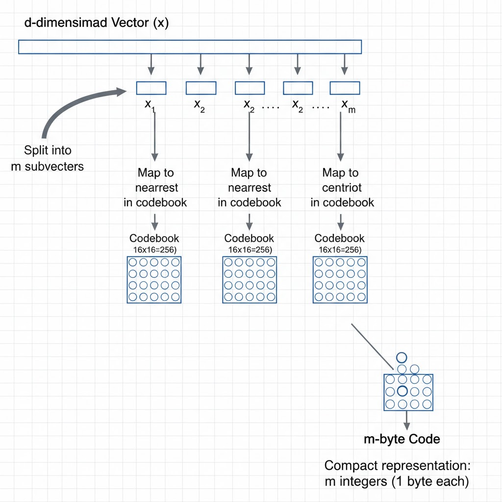 Product quantisation splits vectors into subvectors and encodes each subvector as a byte-sized centroid ID, enabling 32× compression with fast approximate distance via lookup tables.
Product quantisation is a powerful technique for compressing high-dimensional vectors while preserving the ability to compute approximate distances efficiently.
As collections scale past a few million vectors, memory becomes the binding constraint. A 1536-dimensional f32 embedding is 6,144 bytes. Ten million of them occupy ~58 GB, well beyond single-server RAM. Product quantisation (PQ) is the standard technique for compressing vectors by 8–64× with only modest recall degradation.
How PQ works
PQ splits the -dimensional vector into disjoint subvectors of dimensions each:
For each subspace , it trains a separate k-means codebook with 256 centroids (fitting in one byte):
Each vector is then encoded as a sequence of byte-sized centroid IDs:
For and : each subvector has dimensions, the code is 192 bytes. Compression ratio: .
Approximate distance via lookup tables
The power of PQ is not just compression; it also enables fast approximate distance computation. Given a query , precompute a distance table :
This table has entries and costs to build, a one-time cost per query. Then the approximate squared distance between query and any database vector with code is:
This is table lookups and additions, rather than . At vs : 8× fewer operations per distance computation, in addition to the 32× memory saving. The practical result on HNSW is that the inner loop of search_layer (which runs thousands of times per query) becomes massively cheaper.
Asymmetric Distance Computation (ADC): the scheme above keeps the query in full precision and quantises only the database vectors. This is called ADC and is standard in practice; the query stays in full precision since there's only one of them. Symmetric quantisation (also compressing the query) is 32× cheaper still but loses recall rapidly.
Reranking preserves recall
The PQ distances are approximate. To recover precision, the standard pipeline is:
- Run beam search / IVF with PQ distances: fast, low memory, moderate recall.
- Take the top candidates (–).
- Rerank by computing exact distances with the original float32 vectors for just those candidates.
The exact reranking step costs , which is cheap because . The combined recall of this pipeline approaches exact-search recall at a fraction of the memory and compute.