Databases

But, What is a database?#

I've worked with databases for years — PostgreSQL through Supabase, MongoDB for flexible document stores, Redis for caching, and Qdrant for every vector search project I've built. Across all the hackathons I've won and larger systems I've shipped like SparkyAI, there was always a database underneath, and at some point I realized I was using them fluently without really understanding how they worked internally. I knew the APIs, the query languages, the config options — but not the actual engineering underneath.

When I started building Piramid, I went deep. I read Designing Data-Intensive Applications cover to cover, went through database internals papers, and spent a lot of time on buses and between classes just reading about storage engines, indexing structures, and consistency models. This post is that research — a survey of database types I wrote to make sure I actually understood the landscape before building my own. Vector databases don't exist in isolation; they slot into a broader ecosystem, and knowing where other systems stop is how you understand where vector databases begin.

Databases The main families of databases, each built around different assumptions about data shape, access patterns, and the tradeoffs designers were willing to accept.

In-memory databases#

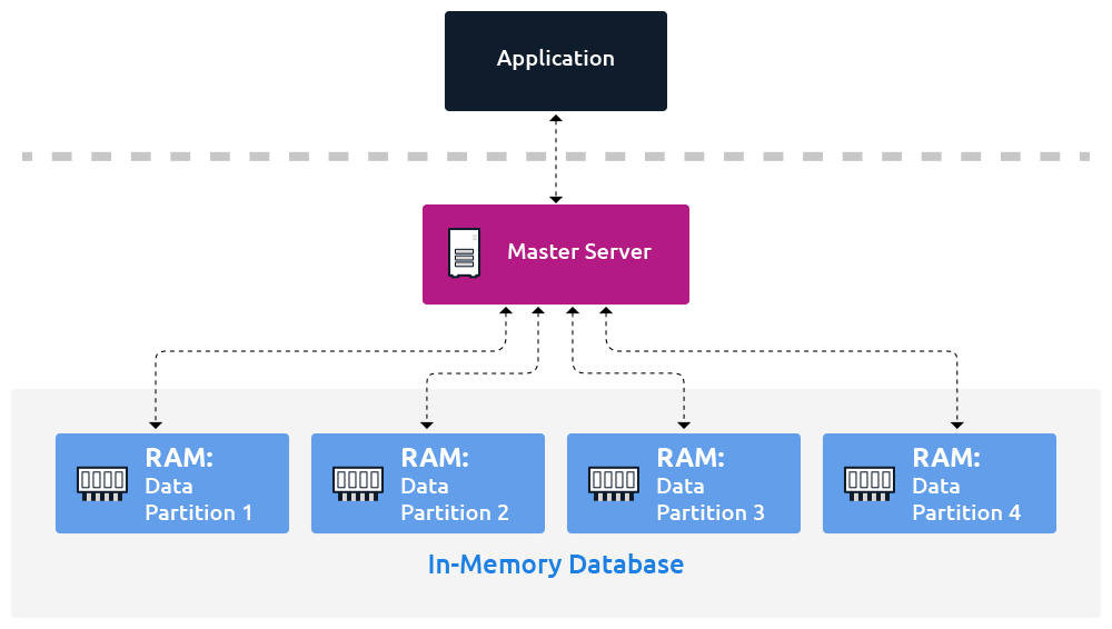In Memory Database An in-memory database keeps all data in RAM, cutting out disk I/O entirely and enabling sub-microsecond latency that disk-backed systems simply can't match.

The premise is simple: instead of reading and writing data to disk, you keep everything in RAM. That sounds obvious until you look at the actual numbers. A RAM access is around 100ns. A random read on a fast NVMe SSD is somewhere between 100μs and 1ms, a factor of $10^3$ to $10^4$ difference, and for workloads doing millions of operations per second, that gap is the entire ballgame.

Most in-memory stores are built on hash tables at their core. A hash function $h: K \to \{0, 1, \ldots, m-1\}$ maps any key to a bucket index, and the value lives at that address in memory. The performance of this hinges on the load factor $\alpha = n/m$, where $n$ is the number of stored entries and $m$ is the number of buckets. With a good hash function and $\alpha$ kept below about 0.7, expected lookup time is $O(1 + \alpha) \approx O(1)$. Let $\alpha$ climb above 1 and collision chains grow, degrading toward $O(n)$ in the worst case, so most implementations either rehash at a threshold or use open addressing with a capped probe distance.

Redis builds on top of hash tables but goes considerably further. A sorted set, for example, is backed by both a hash table ($O(1)$ membership checks by key) and a skip list ($O(\log n)$ range queries by score). A skip list is a probabilistic structure where each node is promoted to a higher level with probability $p = 0.25$, building a tower of linked lists that lets traversal skip large chunks of the sequence. The expected height is $O(\log_{1/p} n)$ and expected search time is $O(\log n)$; for a sorted set with a million members that's about 20 comparisons rather than a million. Streams use a radix tree. Lists compress to a listpack below a size threshold. Each structure was picked because of what the actual access pattern demands, not for uniformity, and understanding that design philosophy reveals a lot about how thoughtful storage systems work in general.

Persistence is where the tradeoffs really show up. Redis offers two strategies: RDB (a periodic fork-and-snapshot to disk, low overhead but can lose a configurable window of writes) and AOF (an append-only log of every write command, recoverable to the last fsync). You can run both simultaneously. But the further you push toward durability, with smaller fsync intervals and more frequent snapshots, the more your latency starts resembling a disk-backed system. At the extreme, AOF with fsync always gives you full durability at the cost of every write being bounded by disk latency, which defeats most of the reason you chose an in-memory store. Nothing is free, and this tension shows up at every layer of the stack.

The constraint that really shapes when you use in-memory storage is cost. At current cloud pricing, 1TB in RAM is roughly 10–20x more expensive than 1TB on NVMe. For hot data that gets read constantly, the latency savings more than justify it. For cold data you touch infrequently, it doesn't. Real systems almost always end up layering (hot working set in memory, warm and cold data on disk), and the design question becomes where those boundaries sit.

Relational databases#

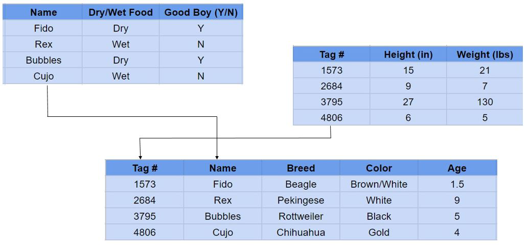Relational database Tables, rows, foreign keys, and SQL — the relational model is still the right default for anything where correctness of data relationships genuinely matters.

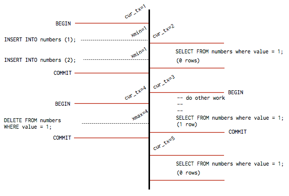how Postgres avoids read-write contention without locking

Relational databases are probably what most people picture when they hear "database." Postgres, MySQL, SQLite: data organized into tables with defined schemas, rows representing individual records, and SQL as the query language. Postgres is the one I've used the most — through Supabase for most of my projects and directly at Decision Theatre where I work on data visualization platforms and implemented B-tree indexing for optimized query pipelines. The relational part is specifically about modeling relationships between entities in separate tables and querying across them with joins.

The core data structure that makes them fast is the B-tree. When you create an index on a column, the database builds a balanced tree where each internal node can hold up to $2t - 1$ keys and $2t$ child pointers, with $t$ being the minimum degree. Postgres uses 8KB pages, fitting hundreds of keys per node. The height of the tree is bounded by:

$h \leq \left\lceil \log_t \frac{n+1}{2} \right\rceil$

For a table with $n = 10^9$ rows and $t = 500$, that works out to $h \leq 4$. Four disk reads to find any record in a billion-row table. Without an index you'd scan all billion. This bound is also why database performance degrades gracefully with table growth; height grows logarithmically, and internal nodes read repeatedly tend to stay hot in the buffer cache.

ACID is the other defining property — and the one I think about most when evaluating whether a data store is actually trustworthy. Atomicity means a transaction either commits fully or rolls back fully; no partial state is visible to anyone. Consistency means every transaction moves the database between valid states, respecting all declared constraints. Isolation means concurrent transactions behave as if they ran serially, which Postgres implements via MVCC (multi-version concurrency control): old row versions remain visible to read transactions while a write is in progress, so readers never block writers and writers don't block readers. Durability means once a commit is acknowledged, the data survives a crash, enforced through a write-ahead log where every change is recorded on disk before it touches the actual data files, making recovery a matter of log replay. These four properties are why relational databases are the default choice for financial systems, user account stores, inventory, anything where correctness of data relationships genuinely matters.

They're also worth understanding because almost every other database type you'll encounter is a reaction to their constraints: rigid schemas, horizontal scaling difficulty, and poor performance when rows are semi-structured blobs of varying shape.

But to understand why the relational model became dominant in the first place, it helps to know what came before it.

Hierarchical databases#

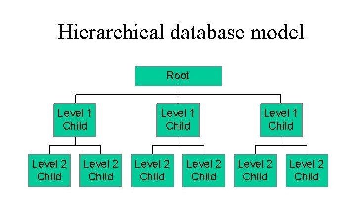Hierarchical Database The hierarchical model organizes data as an inverted tree — fast and simple when the domain is genuinely tree-shaped, brittle the moment you hit a many-to-many relationship.

The hierarchical model predates relational by about a decade. IBM's IMS (Information Management System), developed in 1966 for managing the Apollo program's parts inventory, was one of the first production database systems and it organized data as an inverted tree. Every record (called a segment) has exactly one parent and can have multiple children, and the only way to get to data is by navigating downward from the root. To find an employee's salary you'd traverse: Root → Division → Department → Employee → Salary. If the tree has depth $d$, that retrieval costs $O(d)$ steps, which is fine as long as you know your access path and the tree is shallow.

This maps naturally to domains that are genuinely tree-shaped: organizational hierarchies, bill-of-materials systems, filesystem metadata. The problem surfaces immediately with many-to-many relationships: an employee belonging to multiple projects, a part appearing in multiple assemblies. IMS handles this via "logical" parent pointers that effectively bolt a second tree on top of the first, which works but adds real complexity and means your data model has to anticipate every access pattern you'll ever need, at design time.

The model is more alive today than people realize. LDAP (Lightweight Directory Access Protocol) is hierarchical by definition; every entry has a Distinguished Name that encodes its full path from root (cn=alice,ou=engineering,dc=example,dc=com). The Windows Registry is hierarchical. The HTML/XML DOM is hierarchical. For these specific use cases, the model is exactly right. But it breaks down hard whenever the data's natural structure isn't a tree, and that fragility is what motivated the next step.

Non-relational databases#

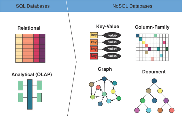NoSQL landscape NoSQL covers a wide range of systems — document, key-value, wide-column, and graph — that share almost nothing except opting out of the relational table model.

NoSQL is a wide umbrella — the systems grouped under it are quite different from each other. The only thing they reliably share is that they don't use the relational table model. The CAP theorem is the clearest lens I've found for understanding why each one is designed the way it is: a distributed system can guarantee at most two of consistency (every read gets the most recent write), availability (every request gets a response), and partition tolerance (the system keeps running during network splits). Since partition tolerance is non-negotiable in any real distributed system, the practical choice is between consistency and availability under partition — and most NoSQL systems explicitly chose availability.

Document databases like MongoDB store data as JSON documents where schema is flexible and fields can vary per document. I've used Mongo extensively — for the GPU infrastructure dashboard I built at AIS where flexible schemas made sense for managing user sessions and runpod configurations that changed shape constantly. Queries translate to B-tree lookups on whatever indexes you've defined, or to a full collection scan otherwise. This is genuinely useful when domain objects have irregular shapes or when schema evolves quickly, but without enforced constraints you lose the correctness guarantees that foreign keys and schema validation provide, and at scale you can end up with inconsistent data in ways that are surprisingly hard to track down.

Key-value stores take the model to its minimum: a key maps to an opaque value and the system knows nothing about the value's internal structure. DynamoDB distributes data using consistent hashing, where the hash space is imagined as a ring of size $2^b$ for some bit-width $b$. Each node is assigned a position on the ring at $h(\text{node\_id})$, and each key routes to the first node clockwise from $h(\text{key})$. The useful property here is that when a node is added or removed, only $n/N$ keys need to move on average (where $n$ is total key count and $N$ is node count), rather than the $O(n)$ remapping a naive modulo scheme would require — which makes scaling incremental rather than disruptive. The cost is narrow expressiveness: no joins, no cross-key scans, no complex filtering.

Wide-column stores like Cassandra are designed for write-heavy distributed workloads. Data is partitioned by a row key and sorted within each partition by a clustering key, with a column-oriented on-disk layout that makes range scans on the clustering key sequential reads. Writes go to a commit log and an in-memory memtable, which flush periodically to immutable SSTables on disk, and reads may span multiple SSTables merged on the fly. Consistency is tunable per operation via quorum: for $N$ replicas, strong consistency requires $W + R > N$, where $W$ is the write quorum and $R$ is the read quorum. A typical setting is $W = R = \lfloor N/2 \rfloor + 1$, giving majority quorum. Drop below that and you get better availability at the cost of potentially stale reads, which is the practical face of CAP under partition.

Graph databases like Neo4j model data as nodes and edges stored as an adjacency list: each node record contains a pointer to its first relationship, and each relationship record points to the next relationship for each endpoint. Traversal follows these pointers directly, making each hop $O(1)$ rather than a B-tree join. For a $k$-hop traversal over a graph with average degree $d$, you touch $O(d^k)$ nodes but each hop costs a constant number of pointer dereferences. In SQL, expressing the same thing requires $k$ self-joins whose cost grows with each added hop and with table size. For problems where the relationships are the data (fraud detection, recommendation graphs, knowledge graphs), this isn't just faster, it's the correct abstraction. The relational model actively fights you when the problem is fundamentally about traversal.

What connects all of these is the same underlying reality: each one traded the generality and correctness guarantees of the relational model for something specific — scale, flexibility, write throughput, or traversal performance. Most operate under BASE (Basically Available, Soft state, Eventually consistent) rather than ACID, and the CAP theorem governs the design space they're all navigating.

What is a vector database?#

This is where my story really begins. I got into AI through an unusual path — I started with agents, then dove deep into RAG while building SparkyAI (where I seriously went down the rabbit hole of reranking mechanisms and advanced RAG variations), then worked backwards into LLMs and transformer architectures through my Advanced Deep Learning class and self-study. Most people go the other way around. But by the time I was building RAG systems for hackathons, I was already a heavy Qdrant user — it was my go-to vector database for everything. I'd read their blogs, understood the config deeply, and used it across every project I shipped.

What made me want to build my own was a combination of things. I saw Helix DB — a new YC-backed vector database — and it clicked that this was exactly the kind of large-scale engineering project I wanted to take on. Not another wrapper or integration, but the actual infrastructure. I'd also been building Kaelum which taught me about neural network routing, and between that and my deep RAG experience I had this thought: what if instead of building wrapper MCPs for databases, I could make the database itself natively smart and optimized for RAG? Auto-adjusted search mechanisms, intelligent index selection — a system that understands what it's doing rather than being a manual machine someone has to tune.

I started thinking about vector databases as a kind of decoupled brain for LLMs — the same way transformers use cosine-based attention and positional embeddings internally, a vector database does something similar but externally, as a separate retrieval memory. That mental model helped me understand both systems more deeply.

But to explain what a vector database actually is: vectors are mathematical representations of data points in a multi-dimensional space. Each vector is a list of numbers (dimensions) that capture characteristics of the data. In NLP, a vector might represent a word or sentence, where each dimension captures some aspect of its meaning.

Vectors illustration Vectors in high-dimensional space: semantically similar inputs cluster nearby, which is what makes similarity search possible and why the geometry of the space matters so much.

A vector database stores and searches these high-dimensional vectors. While traditional databases search for exact matches (finding the exact word "apple" in a text column), vector databases search for semantic similarity — they find data that means the same thing, even if it doesn't look the same. This is the underlying technology powering modern AI, including large language models, recommendation engines, and reverse image searches.

Key Components of a Vector Database System#

A complete vector database involves several parts that have to work together: ingesting data, organizing it for fast retrieval, and answering queries in a way that's both fast and accurate. This is what I found when I opened Excalidraw and started sketching Piramid's architecture — every decision connects to five others. Nothing in database systems is isolated. Each component is worth going through properly, because each has non-obvious depth.

The Embedding Model#

The first step happens before the database even sees the data. Before anything is stored, an AI model processes your raw input (text, images, audio, whatever) and outputs a fixed-length vector. That vector is a dense array of floating point numbers like [0.12, -0.45, 0.89, ...], and the key property is that the model has been trained such that semantically similar inputs produce geometrically nearby vectors in high-dimensional space. The word "dog" and the word "puppy" end up close together; "car" ends up far away. The implication for the database is that it never works directly with text or images; it only ever works with these vectors, and the semantic meaning is entirely a function of the model that produced them. Swap the model and you have to re-embed your entire dataset from scratch, because the geometry of the new space is fundamentally incompatible with the old one.

It's also worth understanding what an embedding actually represents mathematically. A model like text-embedding-3-large maps an arbitrary string to a point in $\mathbb{R}^{3072}$. The training objective shapes that space so that the cosine similarity between two points corresponds to semantic similarity between the original inputs. Dimensions don't have human-interpretable meanings individually; it's the relative geometry across all dimensions together that carries the information. This is why naive dimensionality reduction tends to hurt recall: you can't just drop dimensions and expect the semantic structure to survive.

The Vector Index#

Once vectors are stored, the database needs to answer queries of the form: given a query vector $\mathbf{q} \in \mathbb{R}^d$, find the $k$ stored vectors most similar to it. The brute-force approach (computing a distance between $\mathbf{q}$ and every stored vector) costs $O(nd)$ per query, where $n$ is the number of vectors and $d$ is their dimension. For a million 1536-dimensional vectors, that's over $1.5 \times 10^9$ floating-point operations per query. Too slow for interactive use.

Index structures solve this by organizing vectors so you can prune large portions of the search space before doing any distance computation. HNSW (Hierarchical Navigable Small World) builds a multi-layer proximity graph: the top layer is sparse with long-range edges, and each lower layer is progressively denser. Search starts at the top, greedily follows edges toward the query, drops to a lower layer when it can't improve, and terminates at layer zero with a candidate set. Expected traversal cost is $O(\log n)$. IVF (Inverted File Index) takes a different approach: it partitions the vector space into $k$ Voronoi cells using k-means, and at query time only probes the $nprobe$ nearest cells rather than all of them. If those $nprobe$ cells contain fraction $f$ of the data, the search cost drops from $O(nd)$ to roughly $O(f \cdot nd)$. Both are approximate: they trade a small, configurable amount of recall for a large reduction in compute, which is usually the right tradeoff.

Product Quantization (PQ) is a orthogonal technique that addresses memory rather than search time. It compresses each $d$-dimensional vector by splitting it into $M$ subspaces of dimension $d/M$, quantizing each subspace independently to one of $K$ centroids (typically $K = 256$, fitting in a single byte). A full float32 vector costs $4d$ bytes; after PQ it costs just $M$ bytes, a compression ratio of $4d/M$. For $d = 1536$ and $M = 64$, that's a 96× reduction. The tradeoff is distance approximation error introduced by the quantization, which degrades recall and has to be managed by over-fetching candidates and re-ranking with exact distances.

More on how each index type is selected and tuned in the indexing section.

Distance Metrics#

The distance metric defines what "similar" means — and choosing the wrong one quietly degrades recall in a way that's hard to debug, because the wrong metric still returns results, just slightly worse ones. Three dominate in practice.

Cosine similarity measures the angle between two vectors regardless of their magnitude:

$\text{sim}(\mathbf{a}, \mathbf{b}) = \frac{\mathbf{a} \cdot \mathbf{b}}{\|\mathbf{a}\| \, \|\mathbf{b}\|}$

The result is in $[-1, 1]$, where $1$ means identical direction, $0$ means orthogonal, and $-1$ means opposite. Because it normalizes out magnitude, it's scale-invariant; the length of a document doesn't affect how similar it is to a query, only its direction in embedding space does. That's usually what you want for text.

Euclidean distance (L2) measures the straight-line distance between two points:

$d(\mathbf{a}, \mathbf{b}) = \sqrt{\sum_{i=1}^{d}(a_i - b_i)^2}$

Unlike cosine, this is sensitive to vector magnitude. If your embedding model produces vectors where length encodes meaningful information (certain image or audio embeddings), then L2 is more appropriate. For text embeddings that don't normalize their output norms, L2 and cosine can give meaningfully different rankings.

Dot product computes $\mathbf{a} \cdot \mathbf{b} = \sum_{i=1}^{d} a_i b_i$, which is equivalent to cosine similarity when both vectors are unit-normalized (since $\|\mathbf{a}\| = \|\mathbf{b}\| = 1$ trivially cancels the denominator). Most modern embedding APIs return unit-normalized vectors by default, so in practice dot product and cosine are interchangeable, and dot product is preferred in high-throughput paths because it skips the norm computation entirely. The difference is small per query, but across millions of queries it adds up.

Metadata and Hybrid Search#

A vector by itself is just a string of numbers. What makes retrieved results useful is the metadata stored alongside each vector: the original text, a document ID, an author, a timestamp, a category. Without metadata you'd get back a list of opaque vectors with no way to know what they refer to.

Metadata is also what enables hybrid search — combining a vector similarity constraint with a structured filter like year = 2025 AND category = "research". This sounds straightforward but the implementation is genuinely tricky, and it was one of the harder parts to reason about in Piramid. If you apply the metadata filter before the ANN index, the index only sees a subset of vectors, which breaks the graph connectivity assumptions HNSW was built around and can cause recall to collapse. If you apply it after (letting the ANN return $k$ candidates and then filtering), you may discard most candidates and return fewer than $k$ results to the caller, especially when the filter is selective. The right strategy depends on filter selectivity: post-filtering works well for loose filters, but tight filters need either a filter-aware index traversal or significant over-fetching with a high filter_overfetch multiplier. This is a real operational consideration and something you'll tune in production.

The Query Engine#

The query engine is what ties everything together. It receives the incoming request, decides which index to use, coordinates the ANN search with metadata filtering, applies the chosen distance metric, and returns the top $k$ results ranked by similarity score. It's also the layer that handles concurrency (multiple queries hitting the same collection simultaneously) and enforces any budget constraints like timeouts or complexity limits.

How these pieces interact at the query layer has a bigger impact on real-world latency than most people expect. The index type, the distance metric, the filter strategy, whether vectors are memory-mapped or fully loaded, whether metadata lives inline or in a separate store, all of these are query-time decisions that compound. A well-tuned query engine on a good index will feel instant. A poorly configured one on the same hardware can be 10–100× slower with no obvious reason why.

More on these things in later sections

What does the flow look like in practice?#

Putting it all together: you feed raw text into an embedding model, which outputs a vector. You store that vector alongside its metadata in the vector database, and the database updates its index to place the new vector in the appropriate neighborhood. When a user asks a question, the question is also converted into a vector by the same model. The database runs an ANN search over the index using the chosen distance metric, applies any metadata filters, and returns the top $k$ most similar results — not the ones that exactly match a keyword, but the ones that are semantically closest in the embedding space. That distinction is the whole point.

This is the same pipeline I built and rebuilt across multiple projects with Qdrant before deciding to build it from scratch in Rust. The difference with Piramid is that I want each of these steps to be something the system reasons about, not just executes — auto-selecting the right index, tuning search parameters based on collection characteristics, making the database smart enough to handle the RAG pipeline's needs without manual knob-turning. The rest of these architecture posts go through each component in detail.